Running CITE-seq data

As of Cytomarker v0.2.0, users have the option to run CITE-seq assays (combined protein and RNA measurements) through the application. There are two options for running the CITE-seq assay, which are listed below.

Requirements

Both CITE-seq run options require that filter_human_gene_names in the inst/config.yaml file in the source code be set to no. Visit this section on custom analysis for more information on setting these variables.

Option 1: Run protein and RNA matrices separately or consecutively

Users may wish to run separate, or consecutive, panel runs for the RNA and protein matrices as separate inputs, and directly compare the panel outputs. This has the benefit of keeping the data in isolation, as the counts for both modalities may have fundamentally different distributions, and therefore may be treated differently during the gene search algorithm.

Here is an example of splitting the RNA and protein counts into separate SingleCellExperiment objects after the appropriate transformation is applied (log transform for RNA, and CLR (Centered Log Ratio) for protein). The dataset used can be downloaded here: https://zenodo.org/records/10839852

library(Seurat)
library(SingleCellExperiment)
library(S4Vectors)
library(scater)
library(Matrix)

cite_seq <- readRDS("small_pbmc.rds")

# RNA (from SCT assay)
rna_mat <- GetAssayData(cite_seq, assay = "SCT", layer = "data")

# Protein (ADT)
adt_mat <- GetAssayData(cite_seq, assay = "ADT", layer = "data")

sce_rna <- SingleCellExperiment(
  assays = list(counts = rna_mat))

sce_rna <- computeLibraryFactors(sce_rna)
sce_rna <- logNormCounts(sce_rna)

rna_log <- assay(sce_rna, "logcounts")

sce_rna <- SingleCellExperiment(
  assays = list(logcounts = rna_log))

colData(sce_rna) <- DataFrame(cite_seq@meta.data)

saveRDS(sce_rna, "cite_seq_rna.rds")

clr_transform <- function(mat) {
  mat <- as.matrix(mat)
  log_mat <- log1p(mat)
  
  sweep(
    log_mat,
    2,
    colMeans(log_mat),
    FUN = "-")
}

adt_clr <- clr_transform(adt_mat)

sce_protein <- SingleCellExperiment(
  assays = list(logcounts = adt_clr))

colData(sce_protein) <- DataFrame(cite_seq@meta.data)

saveRDS(sce_protein, "cite_seq_protein.rds")

For running separately, users again have a couple of options. In one instance, completely separate panel design runs for both the RNA nad protein may be executed, and then the overlapping markers may be computed. Alternatively, the user may wish to start with either the RNA or protein assay, build a preliminary panel, and then run this panel on the second dataset, with the added capability of adding or removing genes in the second run.

warning

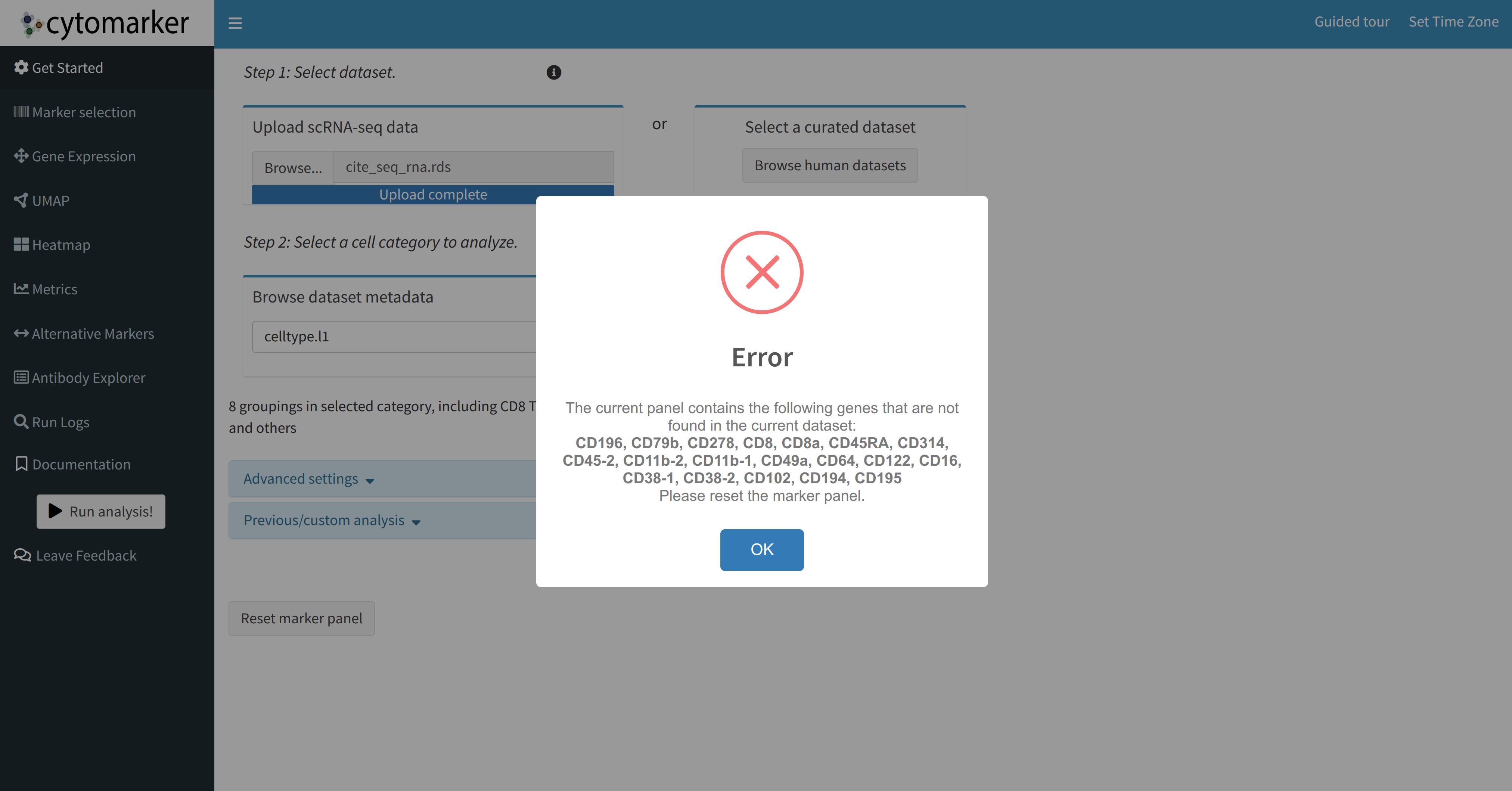
The gene name notation is often different between the RNA and protein assay, so direct comparison of the exact string matches could lead to analytical errors. Further, if a user geneates a preliminary panel with one of the assays, then attempts to re=run analysis with the other assay, to validate the current panel and/or add/remove targets, he/she may get a warning similar to the following:

Option 2: Run concatenated matrix for both modalities with modified gene names

Alternatively, users may choose to concatenate the RNA and protein matrices and run panel generation on both modalities simultaneously. This approach has the benefit of direct comparison of the correlation and expression of genes found in both modalities within the session; however, this also requires manipulation of the gene names so that the user can identify the originating assay that the marker came from (differentiating whether or not the marker is detected in RNA or protein).

As an example, continuing on the example above, we modify the variables names for both assays to have either _protein or _RNA appended to the marker name, ensuring unique variables names once the assays are combined:

# Merge with unique modified gene names
rownames(rna_log) <- paste0(rownames(rna_log), "_RNA")
rownames(adt_clr) <- paste0(rownames(adt_clr), "_protein")

stopifnot(colnames(rna_log) == colnames(adt_clr))

combined_mat <- rbind(rna_log, adt_clr)

sce_combined <- SingleCellExperiment(
  assays = list(logcounts = combined_mat))

colData(sce_combined) <- DataFrame(cite_seq@meta.data)

saveRDS(sce_combined, "cite_seq_combined.rds")

warning

Modifying the marker names with pattern appending as above will cause the antibody catalog explorer to be empty, as the gene symbols will no longer match to the catalog

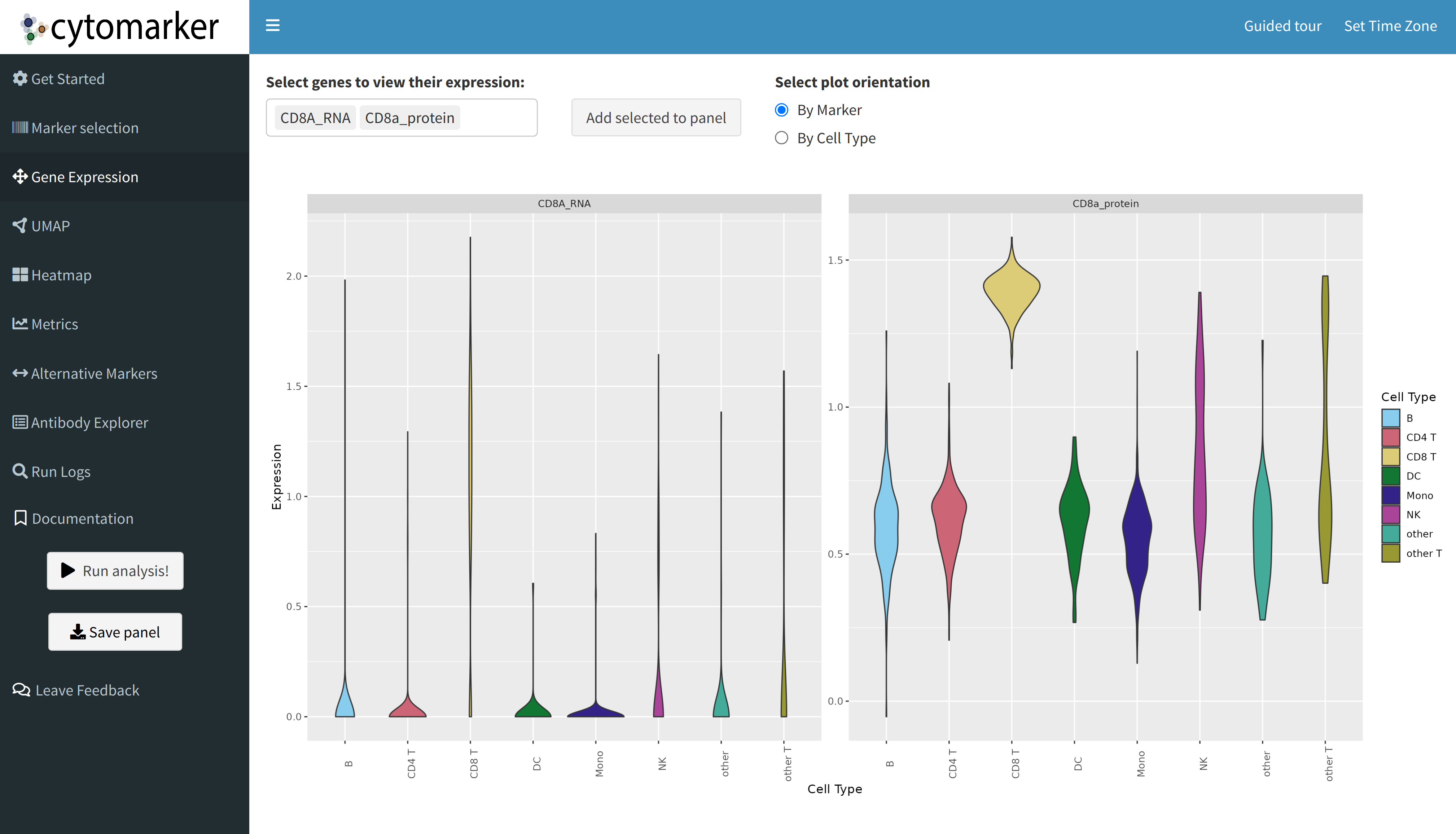
When the assays are run together, Cytomarker's built-in visualization tools such as the violin gene plotting can assist in directly comparing transformed expression for a marker that is found in both modalities:

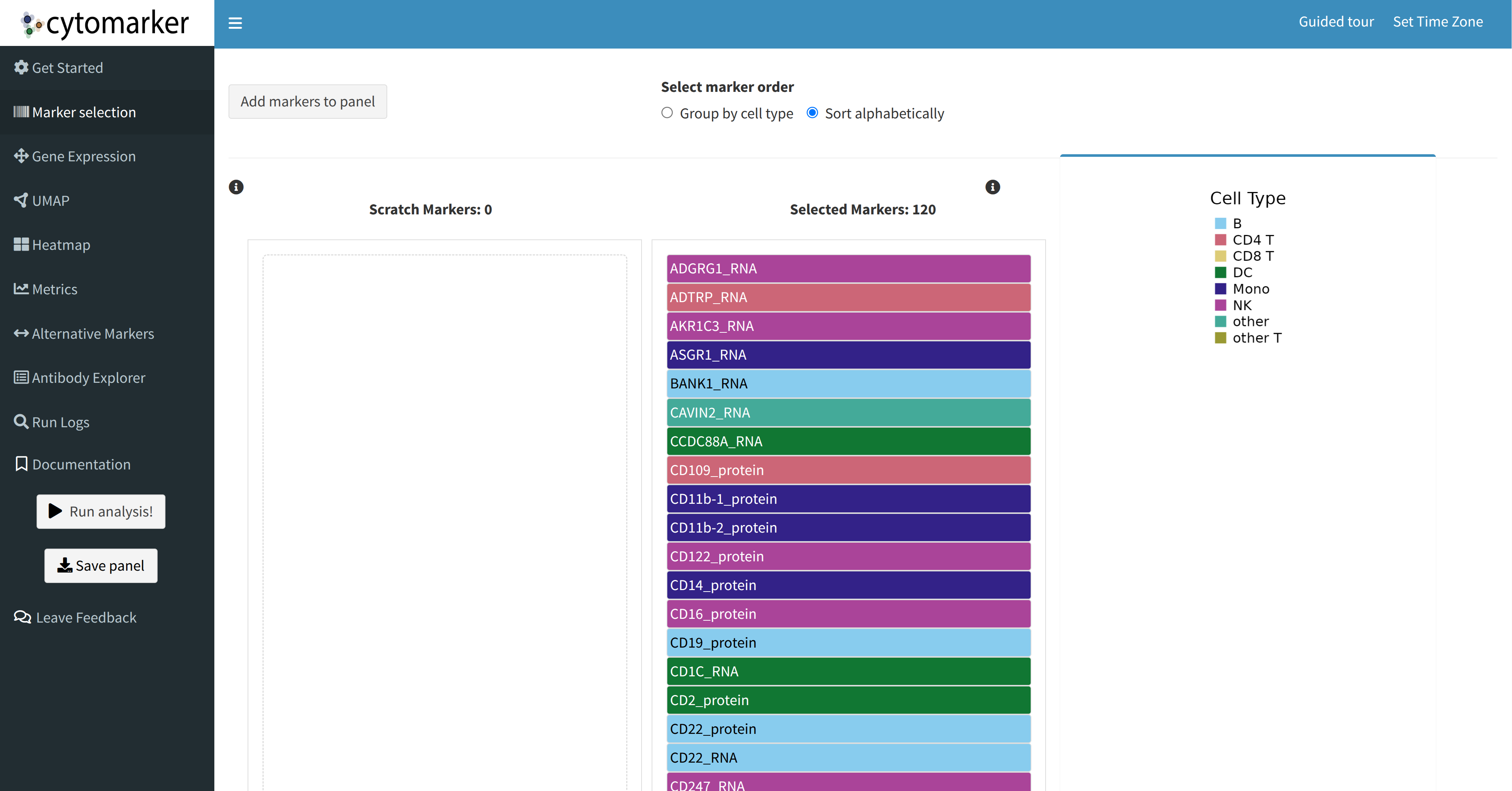
Cytomarker's sorting function for the current panel list can also assist the user in finding targets common to both modalities:

Comparison of approaches

Option 1

• Pros: Keeps genes in isolation, allows for consecutive or separate/parallel runs
• Cons: Panels need to be run separately or compared; lack of gene symbol overlap makes direct comparison of panels difficult

Option 2

• Pros: view both modalities in the same Cytomarker session, leveraging visualization tools for comparison such as violoin gene expression, UMAP, etc.
• Cons: concatenation requires modifying the gene names, making them unlinked to the antibody catalog tab (antibody explorer becomes empty)